机器学习之Logistic回归
Logistic回归
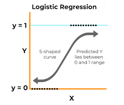
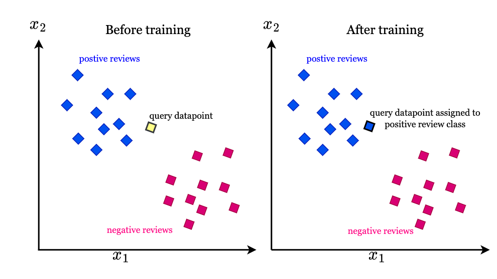
根据现有数据对分类边界线(Decision Boundary)建立回归公式,以此进行分类。
基础概念
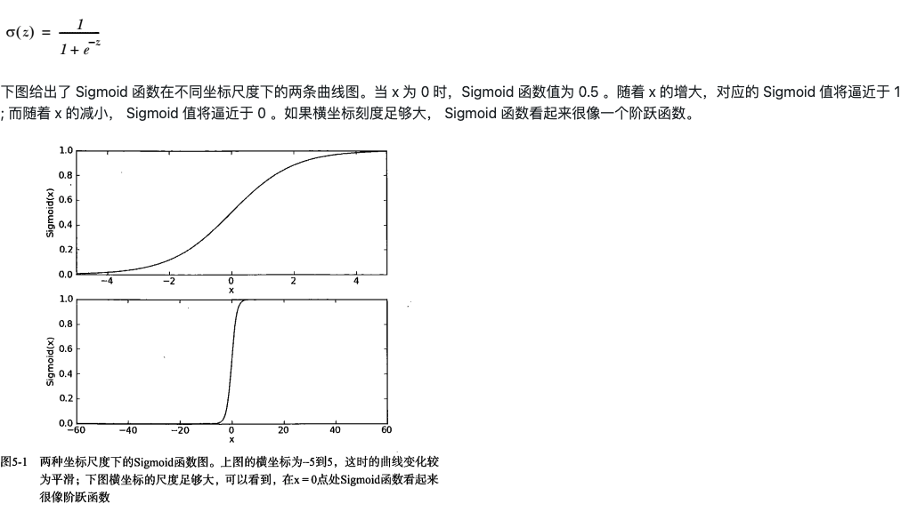
Sigmoid函数
二值型输出分类函数
我们想要函数应该是:能接受所有的输入然后预测出类别。例如,在两个类的情况下,上述函数输出0或1.该函数称为海维赛德阶越函数,或直接称为单位阶越函数。
单位阶越函数的问题在于:该函数在跳跃点上从0瞬间跳跃到1,这个瞬间跳跃的过程有时很难处理。
实现原理
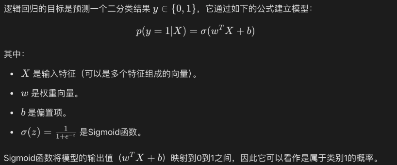
逻辑回归通过使用逻辑函数(Sigmoid函数)将线性回归的输出映射到0和1之间,从而预测某个事件发生的概率。
- 逻辑回归模型
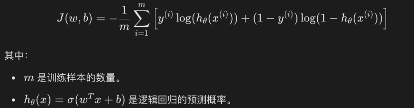
- 损失函数
- 逻辑回归的损失函数是对数损失函数(Log Loss)
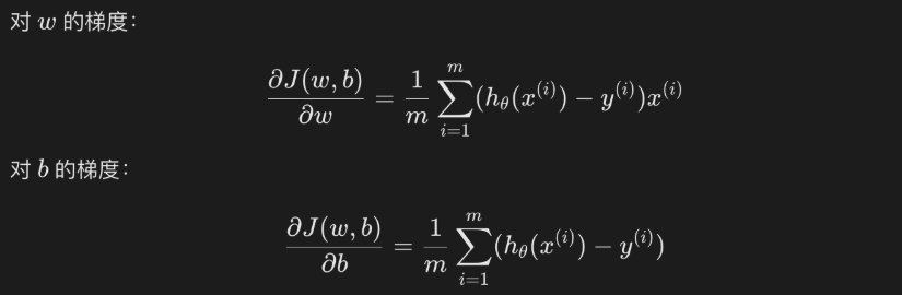
- 梯度下降法求解
- 和线性回归一样,逻辑回归通常也使用梯度下降法来优化损失函数,求解参数w和b
实现代码
1 | import numpy as np |
本博客所有文章除特别声明外,均采用 CC BY-NC-SA 4.0 许可协议。转载请注明来源 廾匸!
相关推荐
2025-06-09
机器学习之KNN
K-近邻算法k-近邻(KNN K-Nearest-Neighbor)knn的输入为样本的特征向量,对应其在特征空间的点;输出为类别。 KNN原理 1.假设有一个带标签的样本数据集(训练样本集),其中包含每条数据与所属分类的对应关系。 2.输入没有标签的新数据后,将新数据的每个特征与样本集中数据对应的特征进行比较。 i.计算新数据与样本数据集中每条数据的距离 计算距离的方式 有很多 这里可以和RAG联系起来 (通常有欧式距离 还可以是minkowski距离或者曼哈顿距离。) ii.对求得的所有距离进行排序(从小到大,越小表示越相似) iii.取前k个样本数据对应的分类标签 KNN算法特点精度高,对异常值不敏感缺点:计算复杂度高,空间复杂度高适用范围:数值型和标称型 小结 如何选择合适对k值? k值小对时候,近似误差小,估计误差大。k值大 近似误差大,估计误差小。 太大太小都不好,可以使用交叉验证(cross validation)来选取合适的k值。(就是挨个试) 实现算法 Brute Force 暴力搜索/线性扫描 KD Tree...
2025-06-10
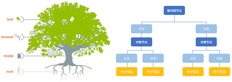
机器学习之决策树
决策树(Decision Tree)是一种基本的分类与回归方法,是最经常使用的数据挖掘算法之一。决策树模型呈树型结构,在分类问题中,表示基于特征对实例进行分类的过程。 决策树学习通常包括3个步骤:特征选择、决策树的生成和决策树的修剪。 基础概念 信息熵&信息增益 熵(entropy):熵指的是体系对混乱程度。 信息论(information theory)中的熵(香农熵):是一种信息的度量方式,表示信息的混乱程度。 信息增益(information...
2025-06-10
机器学习之朴素贝叶斯
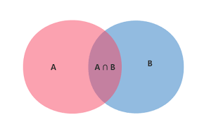
LINK 朴素贝叶斯概述贝叶斯分类算法是统计学的一种概率分类方法,朴素贝叶斯分类(Naive Bayes)是贝叶斯分类中最简单的一种。分类原理:利用贝叶斯公式根据某特征的先验概率计算出其后验概率,然后选择具有最大后验概率的类作为该特征所属的类。朴素:贝叶斯分类只做最原始、最简单的假设:所有特征之间是统计独立的。 相关概念条件概率条件概率(Condittional probability),就是指在事件B发生的情况下,事件A发生的概率,用P(A|B)来表示。 全概率如果事件 A1,A2,…,An 构成一个完备事件且都有正概率,那么对于任意一个事件B则有: 根据条件概率和全概率公式,可以得到贝叶斯公式如下:P(A)称为”先验概率”(Prior probability),即在B事件发生之前,我们对A事件概率的一个判断。P(A|B)称为”后验概率”(Posterior probability),即在B事件发生之后,我们对A事件概率的重新评估。P(B|A)/P(B)称为”可能性函数”(Likely...
2025-06-09
机器学习
(注:博客属个人复习笔记,不会介绍基础概念,仅记录个人遗忘的部分知识点) RUNOBB教程 BLOG教程 机器学习 概述 “机器学习是对能通过经验自动改进的计算机算法的研究” “机器学习是用数据或以往的经验,以此优化计算机程序的性能标准” 机器学习和深度学习的最大区别在神经网络,深度学习使用神经网络去提取事物的深层或者说是隐性的一些特征 常见的模型指标 正确率 —— 提取出的正确信息条数 / 提取出的信息条数 召回率 —— 提取出的正确信息条数 / 样本中的信息条数 F 值 —— 正确率 * 召回率 * 2 / (正确率 + 召回率)(F值即为正确率和召回率的调和平均值) 特征工程 特征选择-也叫特征子集选择(FSS,Feature Subset...