Logistic回归
Logistic回归是一种用于二分类问题的统计学习方法。它通过对输入特征的线性组合结果应用Sigmoid函数,将输出映射到0和1之间,从而预测某个事件发生的概率。与线性回归不同,逻辑回归的输出是概率值,常用于分类任务。
基础概念
Sigmoid函数
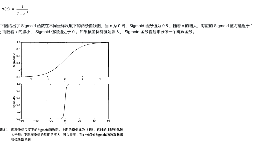
Sigmoid函数是一种常用的激活函数,定义为:
$$
\sigma(z) = \frac{1}{1 + e^{-z}}
$$
它的输出范围在0到1之间,适合用于概率预测。
单位阶跃函数与Sigmoid函数
在二分类问题中,我们希望模型能够根据输入预测类别(0或1)。理想情况下,可以使用单位阶跃函数(Heaviside step function)来实现:
$$
f(x) = \begin{cases}
1, & x \geq 0 \
0, & x < 0
\end{cases}
$$
但由于单位阶跃函数在跳跃点不可导,难以用于优化,因此实际中采用Sigmoid函数作为近似。
实现原理
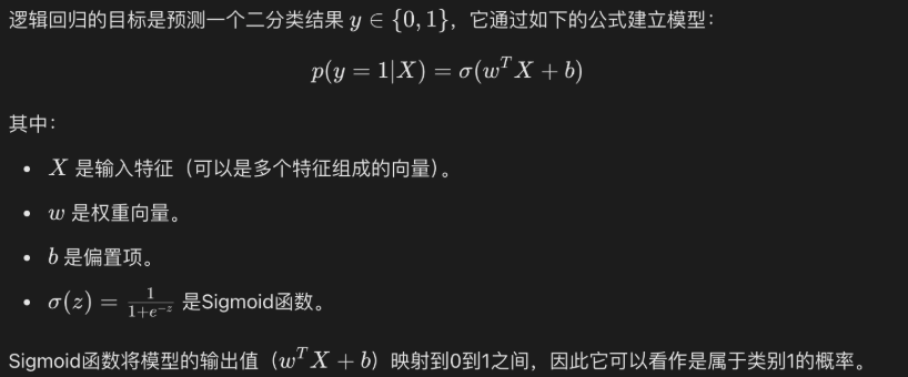
逻辑回归的核心思想是将线性回归的输出通过Sigmoid函数映射到0和1之间,输出表示属于某一类别的概率。
逻辑回归模型公式
$$
P(y=1|x) = \sigma(w^T x + b)
$$
损失函数
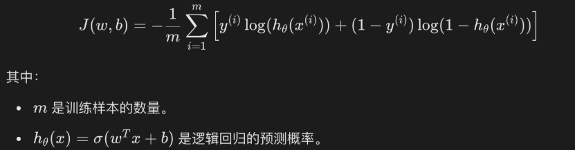
逻辑回归采用对数损失函数(Log Loss):
$$
L = -\frac{1}{m} \sum_{i=1}^{m} [y^{(i)} \log(p^{(i)}) + (1-y^{(i)}) \log(1-p^{(i)})]
$$
参数优化
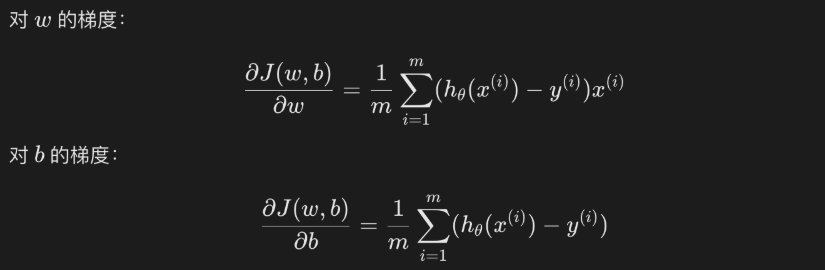
通常使用梯度下降法最小化损失函数,更新参数$w$和$b$。
实现代码
下面是一个使用Python实现的简单逻辑回归模型,基于Iris数据集的前100个样本(仅包含两个类别):
1
2
3
4
5
6
7
8
9
10
11
12
13
14
15
16
17
18
19
20
21
22
23
24
25
26
27
28
29
30
31
32
33
34
35
36
37
38
39
40
41
42
43
44
45
46
47
48
49
50
51
52
53
54
55
56
57
58
59
60
61
62
63
64
65
66
67
68
69
70
71
72
73
74
75
76
77
78
79
80
81
82
83
84
85
86
87
88
89
| import numpy as np
import matplotlib.pyplot as plt
from sklearn.datasets import load_iris
from sklearn.model_selection import train_test_split
iris = load_iris()
X = iris.data[0:100]
Y = iris.target[0:100]
X_train, X_test, y_train, y_test = train_test_split(X, Y, test_size=0.3, random_state=42)
class LogisticRegression:
def __init__(self, learning_rate=0.01, num_iterations=1000):
self.learning_rate = learning_rate
self.num_iterations = num_iterations
self.weights = None
self.bias = None
def sigmoid(self, z):
return 1 / (1 + np.exp(-z))
def initialize_parameters(self, n_features):
self.weights = np.zeros(n_features)
self.bias = 0
def compute_cost(self, X, y, weights, bias):
m = X.shape[0]
z = np.dot(X, weights) + bias
predictions = self.sigmoid(z)
cost = (-1/m) * np.sum(y * np.log(predictions) + (1-y) * np.log(1-predictions))
return cost
def fit(self, X, y):
m, n_features = X.shape
self.initialize_parameters(n_features)
costs = []
for i in range(self.num_iterations):
z = np.dot(X, self.weights) + self.bias
predictions = self.sigmoid(z)
dw = (1/m) * np.dot(X.T, (predictions - y))
db = (1/m) * np.sum(predictions - y)
self.weights -= self.learning_rate * dw
self.bias -= self.learning_rate * db
cost = self.compute_cost(X, y, self.weights, self.bias)
costs.append(cost)
print(f"Iteration {i}, Cost: {cost:.6f}")
return costs
def predict(self, X):
z = np.dot(X, self.weights) + self.bias
predictions = self.sigmoid(z)
return (predictions >= 0.5).astype(int)
def score(self, X, y):
predictions = self.predict(X)
accuracy = np.mean(predictions == y)
return accuracy
model = LogisticRegression(learning_rate=0.1, num_iterations=10)
costs = model.fit(X_train, y_train)
plt.figure(figsize=(10, 6))
plt.plot(range(len(costs)), costs, 'b-', label='Training Loss')
plt.xlabel('Iterations')
plt.ylabel('Cost')
plt.title('Training Loss Curve')
plt.legend()
plt.grid(True)
plt.show()
train_accuracy = model.score(X_train, y_train)
test_accuracy = model.score(X_test, y_test)
print(f"\n训练集准确率: {train_accuracy:.4f}")
print(f"测试集准确率: {test_accuracy:.4f}")
|
回归
回归分析是用于预测连续型目标变量的一类方法。与分类任务不同,回归的目标变量是数值型的。例如,预测房价、温度、销售额等。
回归方程与回归系数
回归模型的核心是回归方程(regression equation),形式如下:
$$
y = w_1 x_1 + w_2 x_2 + \cdots + w_n x_n + b
$$
其中,$w_1, w_2, …, w_n$为回归系数(regression weights),$b$为偏置项。回归系数反映了各特征对目标变量的影响强度。求解回归系数的过程就是回归建模的过程。
一旦得到回归系数,预测新样本时,只需将输入特征与回归系数做加权求和即可得到预测值。
线性回归
线性回归(linear regression)假设特征与目标变量之间存在线性关系。其表达能力很强,可以通过对特征进行函数映射后再线性组合,从而捕捉特征与结果之间的非线性关系。
补充说明:
线性回归不仅可以用于简单的单变量预测,还可以扩展到多元线性回归、带有正则化的岭回归、Lasso回归等多种形式,广泛应用于实际问题中。