OpenCV
OpenCV-图像的基础操作
图像的读取、显示与保存
- 图片的读取与显示使用PIL读取图片
1
2
3
4
5
6
7
8
9
10
import cv2
img = cv2.imread('img_path')
cv2.imshow('windowname',img)
cv2.waitkey(0) # 让窗口持续显示 不会一闪而过
import matplotlib.pyplot as plt
# 因为我用的vscode,更好的图片显示方式是plt
plt.imshow(img)1
2
3
4
5from PIL import Image
image = Image.open(image_path)
image.show()
PIL打开的通道顺序是RGB
opencv打开图片的通道顺序是BGR
shape:
opencv(820,818,3)
PIL(670760,3)
- 图片的保存
cv2.imwrite(‘img_name.jpg’,img)
- 视频的读取与显示
1
2
3
4
5
6
7
8
9import cv2
cap = cv2.VideoCapture('video_path')
while(cap.isOpened()):
ret,frame = cap.read()
cv2.imshow('frame',frame)
if cv2.waitKey(1) & 0xFF == ord('q'):
break
cap.release()
cv2.destroyAllWindows() - 视频的保存 待验证
1
2
3
4
5
6
7
8
9
10
11
12
13
14import cv2
cap = cv2.VideoCapture('video_path')
fourcc = cv2.VideoWriter_fourcc(*'XVID')
out = cv2.VideoWriter('output.avi',fourcc,20.0,(640,480))
while(cap.isOpened()):
ret,frame = cap.read()
if ret == True:
out.write(frame)
cv2.imshow('frame',frame)
if cv2.waitKey(1) & 0xFF == ord('q'):
break
cap.release()
out.release()
cv2.destroyAllWindows()
图像色彩空间
色彩空间转换
1
2
3
4
5
6
7import cv2
src = cv2.imread('img_path')
dst = cv2.cvtColor(src,cv2.COLOR_BGR2GRAY)
cv2.imshow('src',src)
cv2.imshow('dst',dst)
cv2.waitKey(0)
cv2.destroyAllWindows()通道分离
1
2
3
4
5import cv2
img = cv2.imread('img_path')
# b,g,r = cv2.split(img)
img[:,:,0] = 0
cv2.imshow('img',img)HSV色彩空间
HSV色彩 - 色相、飽和度、明度
H的取值0-179,S的取值0-255,V的取值0-255。但是不同的软件的H取值范围不同,如OpenCV取值范围是0-179,Matlab取值范围是0-360。所以当你需要拿opencv的HSV值和matlab的HSV值做比较的时候,需要先做归一化。利用HSV空间提取红色 inRange bitwise_and
1
2
3
4
5
6
7
8
9
10
11
12
13
14
15
16
17
18import cv2
img = cv2.imread('img_path')
hsv = cv2.cvtColor(img,cv2.COLOR_BGR2HSV)
lower_red = np.array([0,100,100])
upper_red = np.array([10,255,255])
# 根据颜色范围定义一个掩码,用于后续的图像处理
# 这里使用cv2.inRange函数来创建一个掩码,掩码将HSV颜色空间中指定范围的像素设置为白色(即255),其余像素设置为黑色(即0)
mask = cv2.inRange(hsv,lower_red,upper_red)
# 应用掩码到原始图像上,只保留掩码中白色(即指定颜色范围)的区域
# 这里使用cv2.bitwise_and函数进行位与操作,将原始图像与掩码进行运算,得到只有指定颜色范围的图像
# 参数img被重复使用,表示对原始图像进行操作,mask参数指明使用之前定义的掩码
res = cv2.bitwise_and(img,img,mask=mask)
cv2.imshow('img',img)
cv2.imshow('mask',mask)
cv2.imshow('res',res)
cv2.waitKey(0)
cv2.destroyAllWindows()得到BGR对应的HSV
1
2
3
4
5
6import cv2
import numpy as np
color = np.uint8([[[24, 19, 214]]])
hsv_color = cv2.cvtColor(color, cv2.COLOR_BGR2HSV)
print(hsv_color)
图形的绘制
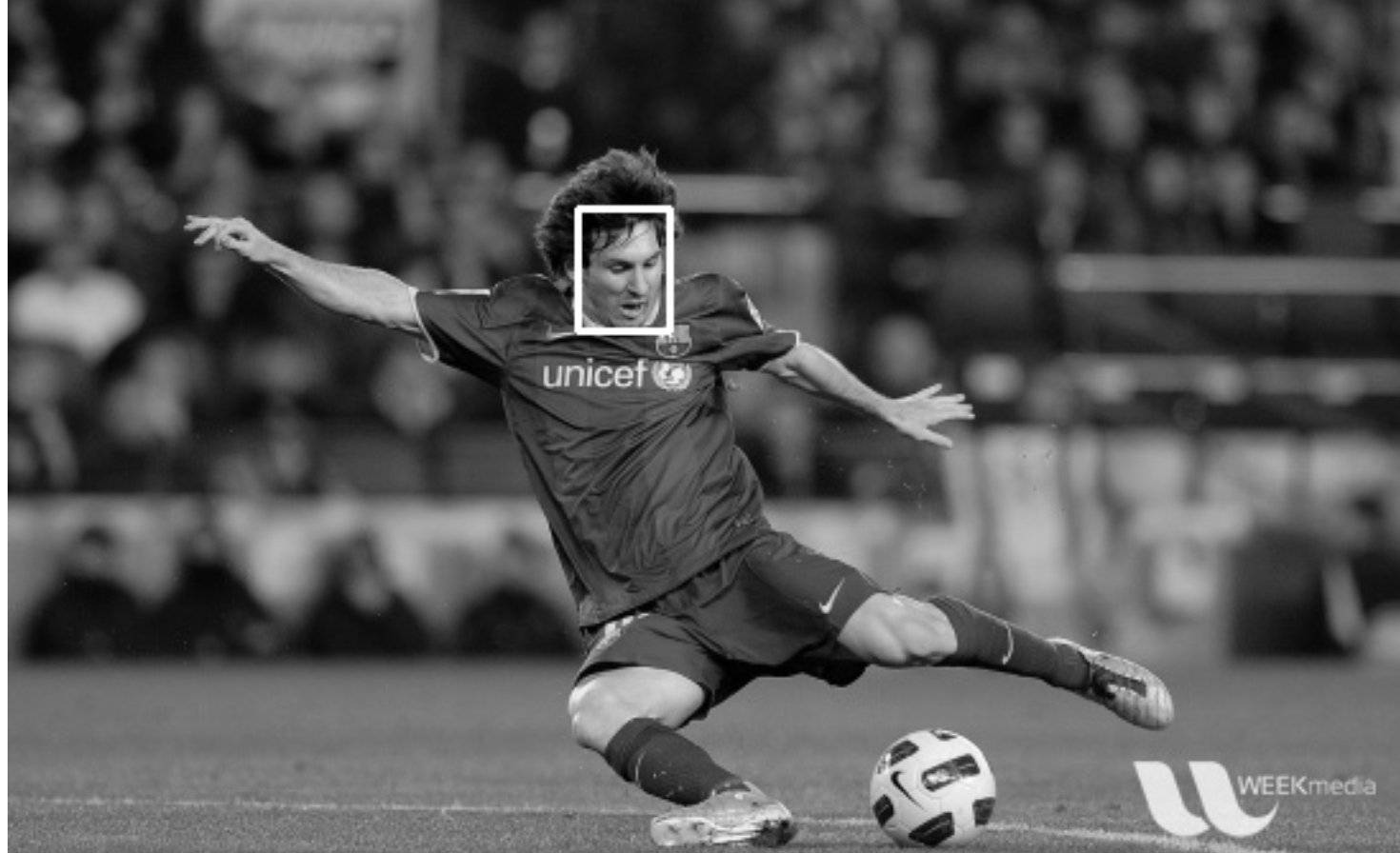
直线、圆、椭圆、矩形
1
2
3
4
5
6
7
8import cv2
img = cv2.imread(r"1.jpg")
# cv2.line(img, (100, 30), (210, 180), color=(0, 0, 255), thickness=2)
# cv2.circle(img, (50, 50), 30, (0, 0, 255), 1)
cv2.rectangle(img,(100,30),(210,180),color=(0,0,255),thickness=2)
# cv2.ellipse(img, (100, 100), (100, 50), 0, 0, 360, (255, 0, 0), -1)
cv2.imshow("pic show", img)
cv2.waitKey(0)多边形 polylines
1
2
3
4
5
6
7
8
9
10import cv2
import numpy as np
img = cv2.imread(r"1.jpg")
# 定义四个顶点坐标
pts = np.array([[10, 5], [50, 10], [70, 20], [20, 30]], np.int32)
# 顶点个数:4,矩阵变成4*1*2维
pts = pts.reshape((-1, 1, 2))
cv2.polylines(img, [pts], True, (0, 0, 255), 2)
cv2.imshow("pic show", img)
cv2.waitKey(0)添加文字 putText
1
2
3
4
5
6import cv2
img = cv2.imread(r"1.jpg")
font = cv2.FONT_HERSHEY_SIMPLEX
cv2.putText(img, 'beautiful girl', (10, 30), font, 1, (0, 0, 255), 1,
lineType=cv2.LINE_AA)
cv2.imshow("pic show", img)cv2.waitKey(0)
OpenCV-高阶操作
阈值操作 threshold
- OTSU二值化操作
1
2
3
4
5
6
7
8
9
10
11
12
13import cv2
img = cv2.imread("1.jpg")
# 将图像转换为灰度图像
# 这一步是为了减少后续处理中对颜色信息的依赖,灰度图像处理起来更简单且计算量更小
gray = cv2.cvtColor(img, cv2.COLOR_BGR2GRAY)
# 应用二值化处理,同时使用OTSU算法自动确定阈值
# 二值化将图像分为黑色和白色两个区域,便于后续的图像分析和处理
# OTSU算法能自动计算最佳阈值,以区分背景和前景,减少人工干预
ret, binary = cv2.threshold(gray, 0, 255, cv2.THRESH_BINARY | cv2.THRESH_OTSU)
cv2.imshow("gray",gray)
cv2.imshow('binary', binary)
cv2.waitKey(0)
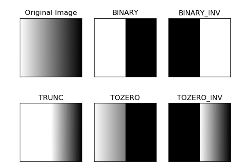
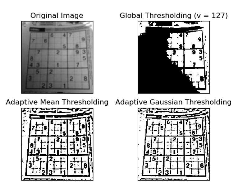
简单阈值
cv2.threshhold() 的第一个参数就是原图像,原图像应该是灰度图。第二个参数就是用来对像素值进行分类的阈值。第三个参数就是当像素值高于(有时是小于)阈值时应该被赋予的新的像素值。OpenCV提供了多种不同的阈值方法,这是有第四个参数来决定的。这些方法包括:
- cv2.THRESH_BINARY
- cv2.THRESH_BINARY_INV
- cv2.THRESH_TRUNC
- cv2.THRESH_TOZERO
- cv2.THRESH_TOZERO_INV
1 | import cv2 |
自适应阈值
当同一幅图像上的不同部分具有不同亮度时,使用自适应阈值。此时的阈值是根据图像上的局部像素值来决定的。
在OpenCV中,可以使用cv2.threshold()函数来执行简单阈值处理,也可以使用cv2.adaptiveThreshold()函数来执行自适应阈值处理。简单阈值处理是指将图像中的像素值与给定的阈值进行比较,如果大于阈值,则将该像素设置为白色(255),否则设置为黑色(0)。自适应阈值处理是指根据图像局部区域的统计信息动态确定阈值,而不是使用固定的阈值。
1 | import cv2 |
图像上的运算
加减法
1
2
3
4
5
6import cv2
import numpy as np
x = np.uint8([250])
y = np.uint8([10])
print(cv2.add(x,y))
print(cv2.subtract(x,y))图像混合
本质上来讲就是加法,只是两幅图的权重不一样,,这就会给人一种混合或者透明的感觉。图像混合
的计算公式如下:g (x) = (1 − α) f0 (x) + α f1 (x)
其中,α 是混合因子,它控制着第一幅图像的权重,而 1 − α 是第二幅图像的权重。dst = α · img1 + β · img2 + γ
这里 γ 的取值为 0。
1 | import cv2 |
- 按位运算
按位运算包括:AND OR NOT XOR1
2
3
4
5
6
7
8
9
10
11
12
13
14
15
16
17
18
19
20
21
22
23
24
25
26
27
28
29
30
31
32import cv2
img1 = cv2.imread('1.jpg')
img2 = cv2.imread('9.jpg')
# 获取输入图像的尺寸
rows, cols, channels = img2.shape
# 从原始图像img1中定义一个与img2相同大小的区域作为感兴趣区域(ROI)
roi = img1[0:rows, 0:cols]
# 将img2转换为灰度图像,为后续处理做准备
img2gray = cv2.cvtColor(img2, cv2.COLOR_BGR2GRAY)
# 使用二值化技术对灰度图像进行处理,生成掩模图像
# 二值化的阈值为10,最大值为255,使用二值化阈值技术
ret, mask = cv2.threshold(img2gray, 10, 255, cv2.THRESH_BINARY)
# 对掩模图像进行取反操作,用于后续的背景提取
mask_inv = cv2.bitwise_not(mask)
# 通过与操作,从ROI中提取出背景部分
img1_bg = cv2.bitwise_and(roi, roi, mask=mask_inv)
# 通过与操作,从img2中提取出前景部分
img2_fg = cv2.bitwise_and(img2, img2, mask=mask)
# 将前景和背景叠加,得到最终的合成图像
dst = cv2.add(img1_bg, img2_fg)
# 将合成图像覆盖到原始图像的ROI区域
img1[0:rows, 0:cols] = dst
cv2.imshow('res', img1)
cv2.waitKey(0)
图像的几何变换
Resize/trainsport/flip
1
2
3
4
5
6
7
8
9
10
11
12
13
14import cv2
import matplotlib.pyplot as plt
src = cv2.imread('01.jpg')
rows, cols, channel = src.shape
dst = cv2.resize(src, (cols * 2, rows * 2), interpolation=cv2.INTER_CUBIC) # 放大
# interpolation参数说明
# INTER_NEAREST - 最邻近插值
# INTER_LINEAR - 双线性插值,如果最后一个参数你不指定,默认使用这种方法
# INTER_AREA -区域插值
# INTER_CUBIC - 4x4像素邻域内的双立方插值
# INTER_LANCZOS4 - 8x8像素邻域内的Lanczos插值
dst = cv2.transpose(src)# 旋转
dst = cv2.flip(src, 0)# 翻转
plt.imshow(dst)仿射变换
任意一个二维图像,我们乘以一个仿射矩阵,就能得到仿射变换后的图像。变换包含:缩放、旋转、平
移、倾斜、镜像。
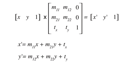
线性代数中的矩阵运算,细看就能看懂。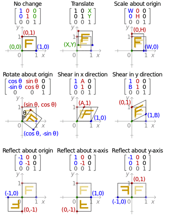
1 | import cv2 |
透视变换(Perspective Transformation)是指利用透视中心、像点、目标点三点共线的条件,按透视旋转定律使承影面(透视面)绕迹线(透视轴)旋转某一角度,破坏原有的投影光线束,仍能保持承影面上投影几何图形不变的变换。简而言之,就是将一个平面通过一个投影矩阵投影到指定平面上。
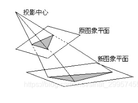
重要的是变换矩阵的计算
1 | #计算变换矩阵 |
腐蚀膨胀操作
- 膨胀操作可以让颜色值大的像素变得粗壮,膨胀之前需要二值化图像。
1 | import cv2 as cv |
- 腐蚀操作可以让颜色值大的像素变得更细,腐蚀前也需要二值化图像。
1 | import cv2 as cv |
开闭运算
开操作是先腐蚀再膨胀,开操作可以用于去噪 MORPH_OPEN
1 | import cv2 as cv |
闭操作是先膨胀再腐,闭操作可以用于补漏洞 MORPH_CLOSE
1 | import cv2 as cv |
梯度操作
膨胀减去腐蚀
1 | import cv2 as cv |
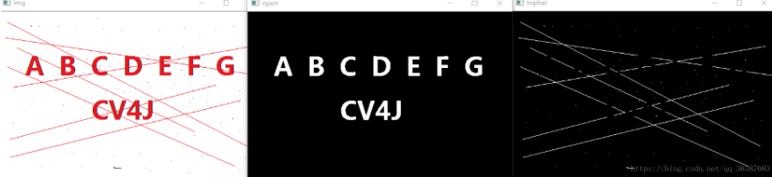
顶帽与黑帽
- 礼帽,是原始图像与进行开运算之后得到的图像的差。
因为开运算到来的结果是放大了裂痕或者局部低亮度的区域,因此,从原图中减去运算后的图,得到的效果图突出了比原图轮廓周围的区域更明亮的区域,且这一操作和选择的核的大小相关。
顶帽运算往往用来分离比邻近点亮一些的斑块。当一幅图像具有大幅的背景的时候,而微小物品比较有规律的情况下,可以使用顶帽运算进行背景提取。
1 | import cv2 as cv |
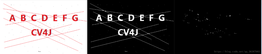
- 黑帽,是进行闭运算之后得到的图像与原始图像的差。
黑帽运算之后的效果图突出了与原图像轮廓周围的区域更暗的区域,且这一操作和选择的核大小相关。所以黑帽运算用来分离比邻近点暗一些的斑块。
1 | import cv2 as cv |
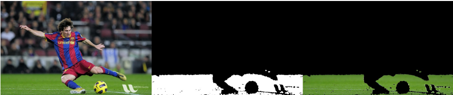
OpenCV-图像分割
图像分割
cv2.watershed()
原理:
- 任何一副灰度图像都可以被看成拓扑平面,灰度值高的区域可以被看成是山峰,灰度值低的区域可 以被看成是山谷。我们向每一个山谷中灌不同颜色的水。随着水的位的升高,不同山谷的水就会相遇汇合,为了防止不同山谷的水汇合,我们需要在水汇合的地方构建起堤坝。不停的灌水,不停的构建堤坝知道所有的山峰都被水淹没。我们构建好的堤坝就是对图像的分割。这就是分水岭算法的 背后哲理。
- 但是这种方法通常都会得到过度分割的结果,这是由噪声或者图像中其他不规律的因素造成的。为了减少这种影响,OpenCV 采用了基于掩模的分水岭算法,在这种算法中我们要设置那些山谷点会汇合,那些不会。这是一种交互式的图像分割。我们要做的就是给我们已知的对象打上不 同的标签。如果某个区域肯定是前景或对象,就使用某个颜色(或灰度值)标签标记它。如果某个区域肯定不是对象而是背景就使用另外一个颜色标签标记。而剩下的不能确定是前景还是背景的区域就用 0 标记。这就是我们的标签。然后实施分水岭算法。每一次灌水,我们的标签就会被更新,当两个不同颜色的标签相遇时就构建堤坝,直到将所有山峰淹没,最后我们得到的边界对象(堤坝)的值为 -1。
1
2
3
4
5
6
7
8
9
10
11
12
13
14
15
16
17
18
19
20
21
22
23
24
25
26
27import numpy as np
import cv2
from matplotlib import pyplot as plt
img = cv2.imread('1.jpg')
gray = cv2.cvtColor(img, cv2.COLOR_BGR2GRAY)
ret, thresh = cv2.threshold(gray, 0, 255, cv2.THRESH_BINARY_INV |
cv2.THRESH_OTSU)
# noise removal
kernel = np.ones((3, 3), np.uint8)
opening = cv2.morphologyEx(thresh, cv2.MORPH_OPEN, kernel, iterations=2)
# sure background area
sure_bg = cv2.dilate(opening, kernel, iterations=3)
dist_transform = cv2.distanceTransform(opening, 1, 5)
ret, sure_fg = cv2.threshold(dist_transform, 0.7 * dist_transform.max(), 255, 0)
# Finding unknown region
sure_fg = np.uint8(sure_fg)
unknown = cv2.subtract(sure_bg, sure_fg)
# Marker labelling
ret, markers1 = cv2.connectedComponents(sure_fg)
# Add one to all labels so that sure background is not 0, but 1
markers = markers1 + 1
# Now, mark the region of unknown with zero
markers[unknown == 255] = 0
markers3 = cv2.watershed(img, markers)
img[markers3 == -1] = [255, 0, 0]
cv2.imshow("img", img)
cv2.waitKey(0)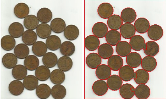
OpenCV-图像滤波
图像滤波
保留图像细节特征的条件下对目标图像的噪声进行抑制
滤波的概念
- 滤波过程就是把不需要的信号频率去掉的过程
- 滤波操作一般用卷积操作来实现,卷积核一般称为滤波器
- 滤波分:低通滤波,高通滤波,中通滤波,阻带滤波
- 低通滤波也叫平滑滤波,可以使图像变模糊,主要用于去噪
- 高通滤波一般用于获取图像边缘、轮廓或梯度
- 中通滤波一般用于获取已知频率范围内的信号
- 阻带滤波一般用于去掉已知频率范围内的信号
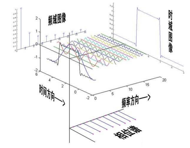
- 滤波分析一般有时域分析和频域分析
- 时域分析是直接对信号本身进行分析
- 频域分析师对型号的变化快慢进行分析
卷积操作
1 | kernel = np.array([[1, 1, 0], [1, 0, -1], [0, -1, -1]], np.float32) # 定义一个核 |
平滑操作
- 均值滤波
1
dst = cv2.blur(src, (5,5))
- 高斯滤波
1
dst = cv2.GaussianBlur(src, (5, 5), 0)
- 中值滤波双边滤波
1
dst = cv2.medianBlur(src, 5)
1
dst = cv2.bilateralFilter(src,9,75,75)
锐化操作
提高图像的锐利程度,使图像变得更清晰
- Laplacian锐化
1
2
3
4
5
6
7
8
9
10
11
12
13
14
15kernel = np.array([[0, -1, 0], [-1, 5, -1], [0, -1, 0]], np.float32) #定义一个核 五领域?
# 使用二维滤波器对图像进行滤波
#
# 该行代码应用了二维滤波器(kernel)对输入图像(src)进行滤波处理,生成的结果图像(dst)。
# 这一操作可以用于平滑图像、边缘检测、特征提取等目的。
#
# 参数:
# - src: 输入图像,可以是灰度图像或彩色图像。
# - -1: 指定输出图像的深度为与输入图像相同。
# - kernel: 用于滤波的核数组,定义了滤波器的特性。
#
# 返回值:
# - dst: 应用滤波器处理后的输出图像。
dst = cv2.filter2D(src, -1, kernel=kernel) - USM锐化
1
2
3
4
5
6
7
8
9dst = cv2.GaussianBlur(src, (5, 5), 0)
# 加权融合源图像和目标图像
#
# 通过加权合并源图像(src)和目标图像(dst),实现图像的融合处理。这种处理常用于图像叠加、透明效果处理等场景。
# 参数src表示源图像,dst表示目标图像。alpha参数为源图像的权重,这里设置为2,表示源图像的贡献较大。
# beta参数为目标图像的权重,这里设置为-1,表示目标图像的贡献由gamma参数来调整。
# gamma参数为调整后的贡献值,这里设置为0,表示不进行额外的贡献值调整。
# 函数返回加权融合后的图像。
dst = cv2.addWeighted(src, 2, dst, -1, 0)
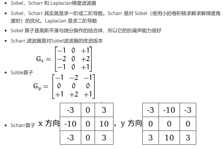
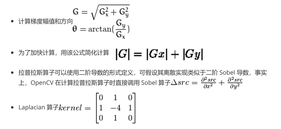
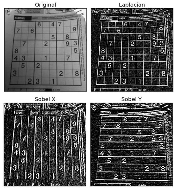
梯度操作
1 | import cv2 |
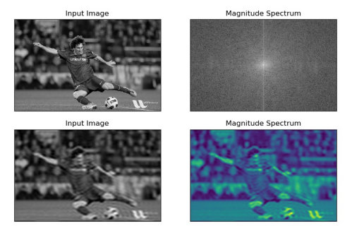
傅里叶变换
- numpy中的傅里叶变换
1 | import cv2 |
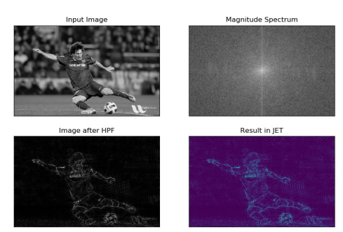
- opencv傅里叶变换
1 | import cv2 |
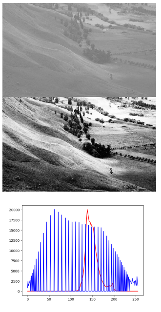
直方图均衡化
直方图均衡化是图像处理领域中利用图像直方图对对比度进行调整的方法。这种方法通常用来增加许多图像的全局对比度,尤其是当图像的有用数据的对比度相当接近的时候。通过这种方法,亮度可以更好地在直方图上分布。这样就可以用于增强局部的对比度而不影响整体的对比度,直方图均衡化通过有效地扩展常用的亮度来实现这种功能。
1 | import cv2 |
自适应均衡化:
1 | import cv2 |
直方图反向投影:
可以用来做图像分割,或者在图像中找到我们感兴趣的部分,简单来说,它会输出与输入图像(待搜索)同样大小的图像,其中的每一个像素值代表了输入图像上对应点属于目标对象的概率。用更简单的话来解释,输入图像中像素值越高(越白)的点就越可能代表我们要搜索的目标(在输入图像所在的位置)。这是一个直观的解释。直方图投影经常与camshift算法等一起使用。
我们要查找的对象要尽量占满这张图(换句话说,这张图像上最好是有且仅有我们要查找的对象)。最好使用颜色直方图,因为一个物体的颜色要比它的灰度更能更好的用来进行图像分割和图像识别。接着我们再把这个颜色直方图投影到输入图像中寻找我们的目标,也就是找到输入图像中的每一个像素点的像素值在直方图对应的概率,这样我们就得到了一个概率图像,最后设置适当的阈值对概率图进行二值化
1 | import cv2 |
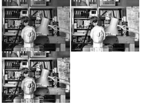
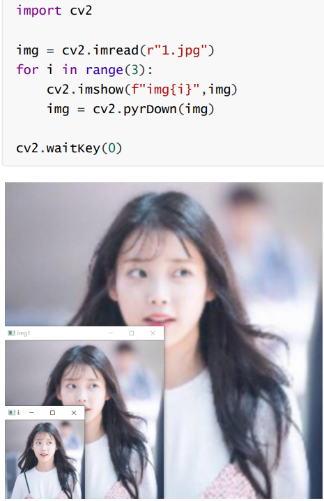
图像金子塔
-上采样和下采样的目的与原理
上采样和下采样是图像处理中的两个重要操作,主要用于改变图像的分辨率。上采样通过增加像素点来放大图像,而下采样则通过减少像素点来缩小图像。
- cv2.pyrUp()
该函数用于对图像进行上采样,即将图像的分辨率增加一倍。它通过插入像素值的平均值来实现放大。
参数说明:
src:输入的图像,可以是单通道或多通道的灰度图像或彩色图像。
dst:输出的图像,大小为输入图像的两倍。
dstsize:输出图像的大小,如果不指定,则默认为输入图像大小的两倍。
borderType:用于指定像素值的复制方式,可以是默认的边界模式。
返回值说明:返回经过上采样后的图像。
- cv2.pyrDown()
该函数用于对图像进行下采样,即将图像的分辨率减小一半。它通过将相邻的像素值平均来实现图像的缩小。
参数说明:
src:输入的图像,可以是单通道或多通道的灰度图像或彩色图像。
dst:输出的图像,大小为输入图像的一半。
dstsize:输出图像的大小,如果不指定,则默认为输入图像大小的一半。
borderType:用于指定像素值的复制方式,可以是默认的边界模式。
返回值说明
返回经过下采样后的图像。
这两个函数在图像处理和计算机视觉中广泛应用,例如在图像金字塔的构建、图像的下采样和上采样等场景中。
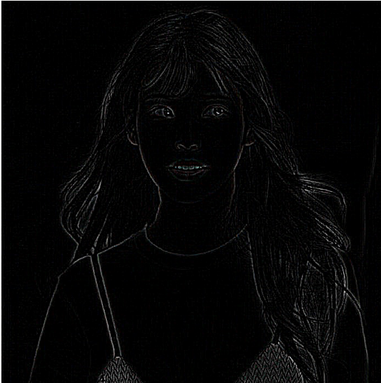
高斯金字塔
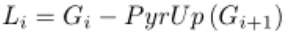
拉普拉斯金子塔
1 | import cv2 |
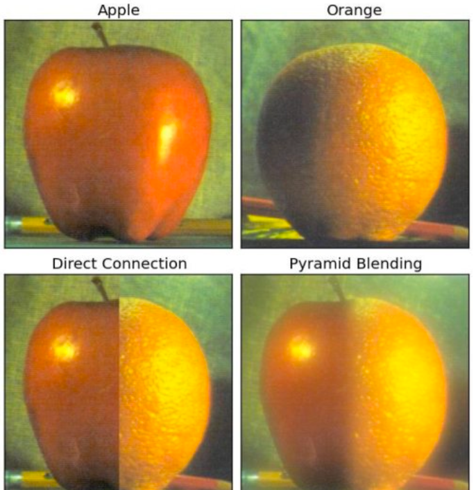
- 图像金字塔还可以用来做图片融合
无缝融合
融合步骤
- 读入两幅图像,苹果和橘子
- 构建苹果和橘子的高斯金字塔(6 层)
- 根据高斯金字塔计算拉普拉斯金字塔
- 在拉普拉斯的每一层进行图像融合(苹果的左边与橘子的右边融合)
- 根据融合后的图像金字塔重建原始图像
1 |
|
OpenCV-模版匹配
模版匹配
单目标匹配
1 | import cv2 |
多目标匹配
1 | import cv2 |

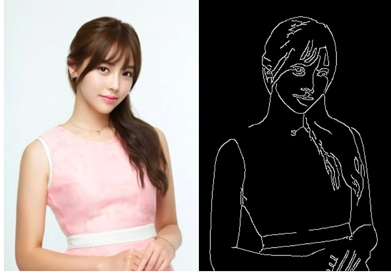
Canny边缘提取算法
1 | import cv2 |
轮廓
轮廓的查找与绘制
1 | import cv2 |
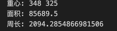
面积、周长、重心
1 | import cv2 |
轮廓近似
将轮廓形状近似到另外一种由更少点组成的轮廓形状,新轮廓的点的数目由设定的准确度来决定。
1 | import cv2 |
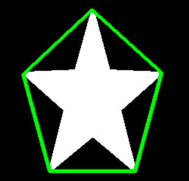
凸包与凸性检测 convexHull
凸包与轮廓近似相似,但不同,虽然有些情况下它们给出的结果是一样的。
函数 cv2.convexHull() 可以用来检测一个曲线是否具有凸性缺陷,并能纠正缺陷。一般来说,凸性曲线总是凸出来的,至少是平的。如果有地方凹进去了就被叫做凸性缺陷。
函数 cv2.isContourConvex() 可以可以用来检测一个曲线是不是凸的。它只能返回 True 或 False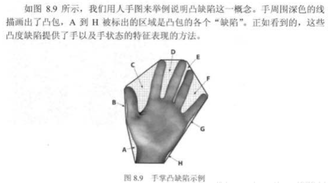
1 | import cv2 |
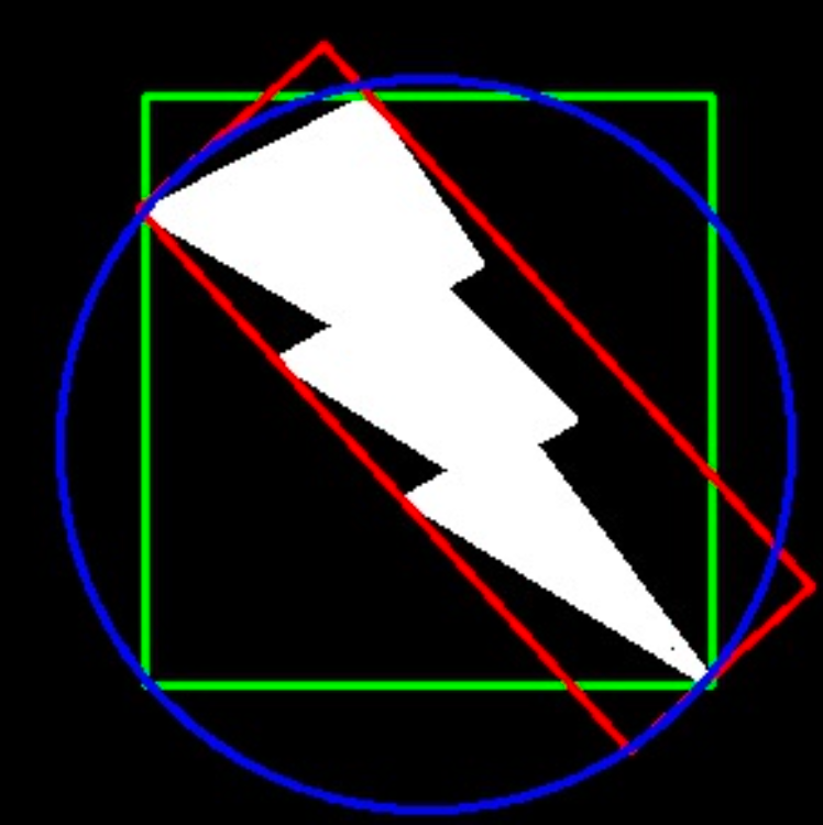
边界检测
1 | import cv2 |
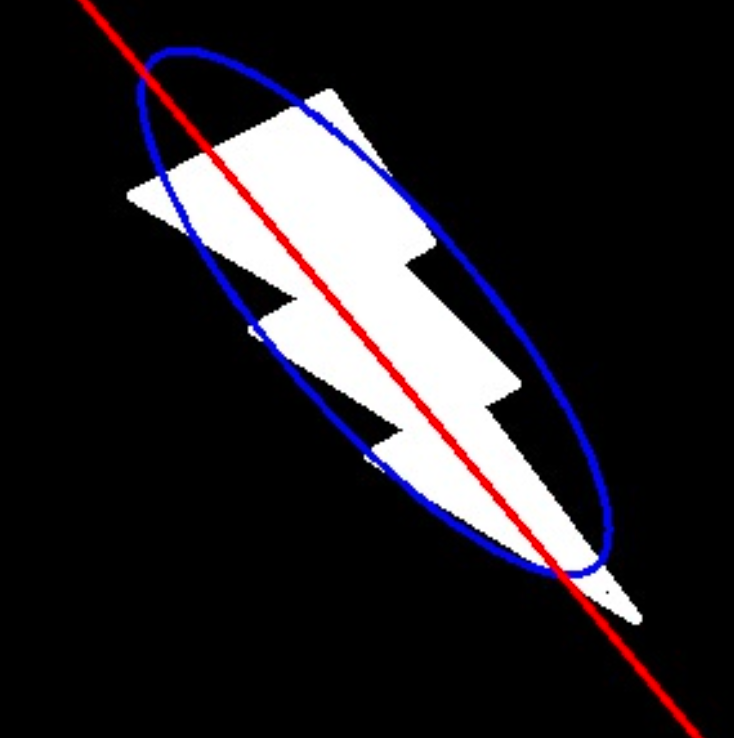
拟合
1 | import cv2 |
轮廓性质
- 边界矩形的宽高比
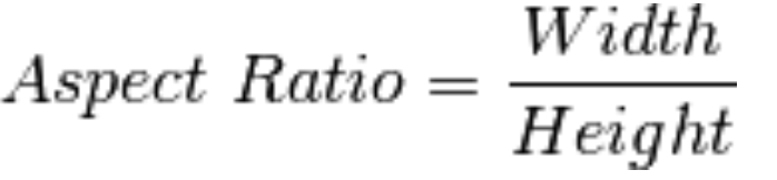
1
2x,y,w,h = cv2.boundingRect(cnt)
aspect_ratio = float(w)/h - 轮廓面积与边界矩形面积的比
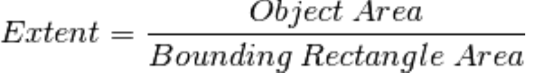
1
2
3
4area = cv2.contourArea(cnt)
x,y,w,h = cv2.boundingRect(cnt)
rect_area = w*h
extent = float(area)/rect_area - 轮廓面积与凸包面积的比
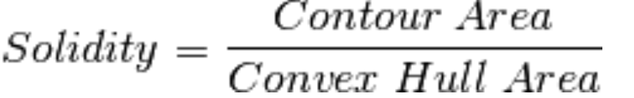
1
2
3
4
area = cv2.contourArea(cnt)
hull = cv2.convexHull(cnt)
hull_area = cv2.contourArea(hull)
solidity = float(area)/hull_area - 与轮廓面积相等的圆形的直径
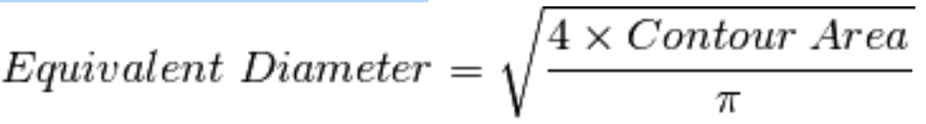
1
2
area = cv2.contourArea(cnt)
equi_diameter = np.sqrt(4*area/np.pi) - 对象的方向
1
2
3
# 通过最小二乘法拟合椭圆
# 参数cnt是轮廓点的集合,函数返回椭圆的中心点坐标(x, y)、长轴和短轴的长度(MA, ma)以及旋转角度angle
(x, y), (MA, ma), angle = cv2.fitEllipse(cnt)
对象的掩码
掩码mask:控制着处理感兴趣区域ROI,region of interest。掩码通常是一个二值图像,像素值为0表示不关心的区域,非0(通常是255)表示感兴趣的区域,通过应用掩码,我们可以将处理限制在感兴趣的区域内,从而提高处理效率并实现更精确的控制。
1 | import cv2 |
- 最大值最小值以及它们的位置
1
min_val, max_val, min_loc, max_loc = cv2.minMaxLoc(imgray,mask = mask)
- 使用相同的掩模求一个对象的平均颜色或平均灰度
1
min_val, max_val, min_loc, max_loc = cv2.minMaxLoc(imgray,mask = mask)
形状匹配
1 | img1 = cv2.imread('4.jpg', 0) |
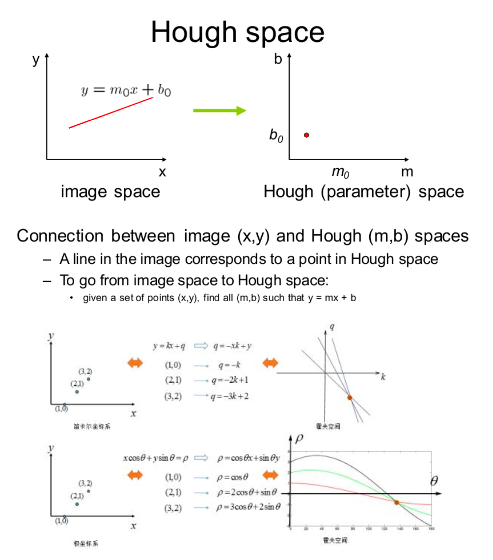
OpenCV-Hough变换
Hough变换
直线检测
1 | import cv2 |
圆检测
1 | import cv2 |
原理:
- 轮廓检测算法检测出轮廓
- 投射到hough空间进行形状检测
数学原理